Unsupervised Learning

Lecture 33

Dr. Eric Friedlander

College of Idaho
CSCI 2025 - Winter 2026

Unsupervised Learning

Machine Learning: using computers and algorithms to learn from data.
Two types of machine learning problems are:
- Supervised Learning: you have a target variable that you’re trying to predict
- Unsupervised Learning: you don’t have a target variables and you’re trying to extract patterns from data
Two common types of unsupervised learning are:
- Dimensionality reduction: find a lower-dimensional representation of the data that captures most of the variation (PCA)
- Clustering: find subgroups of observations that are similar to each other

K-means Clustering

A simple and popular clustering method.
Goal: Partition data into \(K\) distinct, non-overlapping clusters.

How it Works

An iterative algorithm :
1. Initialize: Randomly select \(K\) data points as initial cluster centroids.
2. Assign: Assign each data point to the nearest centroid, forming K clusters.
3. Update: Recalculate the centroid of each cluster (the mean of all points in the cluster).
4. Repeat: Repeat “Assign” and “Update” steps until cluster assignments stop changing.

`tidyclust`

The tidyclust package provides a tidymodels-like interface for clustering.

library(tidymodels)
library(tidyclust)
library(tidyverse)

The Data: `USArrests`

Contains statistics for the 50 US states in 1973:
- Arrests per 100,000 residents for Assault, Murder, and Rape.
- Percent of the population living in urban areas.

USArrests |> head()

           Murder Assault UrbanPop Rape
Alabama      13.2     236       58 21.2
Alaska       10.0     263       48 44.5
Arizona       8.1     294       80 31.0
Arkansas      8.8     190       50 19.5
California    9.0     276       91 40.6
Colorado      7.9     204       78 38.7

K-means with `tidyclust`

Create a k_means() model specification.
Set the number of clusters (k=2 for this example).
Set the engine to "stats".

kmeans_spec <- k_means(num_clusters = 2) |>
  set_engine("stats")

kmeans_spec

K Means Cluster Specification (partition)

Main Arguments:
  num_clusters = 2

Computational engine: stats

K-means with `tidyclust`

Then we can fit the specification.
We are using a formula ~ . to specify that we want to use all variables.

kmeans_fit <- kmeans_spec |>
  fit(~., data = USArrests)

kmeans_fit

tidyclust cluster object

K-means clustering with 2 clusters of sizes 21, 29

Cluster means:
     Murder  Assault UrbanPop     Rape
2 11.857143 255.0000 67.61905 28.11429
1  4.841379 109.7586 64.03448 16.24828

Clustering vector:
       Alabama         Alaska        Arizona       Arkansas     California 
             1              1              1              1              1 
      Colorado    Connecticut       Delaware        Florida        Georgia 
             1              2              1              1              1 
        Hawaii          Idaho       Illinois        Indiana           Iowa 
             2              2              1              2              2 
        Kansas       Kentucky      Louisiana          Maine       Maryland 
             2              2              1              2              1 
 Massachusetts       Michigan      Minnesota    Mississippi       Missouri 
             2              1              2              1              2 
       Montana       Nebraska         Nevada  New Hampshire     New Jersey 
             2              2              1              2              2 
    New Mexico       New York North Carolina   North Dakota           Ohio 
             1              1              1              2              2 
      Oklahoma         Oregon   Pennsylvania   Rhode Island South Carolina 
             2              2              2              2              1 
  South Dakota      Tennessee          Texas           Utah        Vermont 
             2              1              1              2              2 
      Virginia     Washington  West Virginia      Wisconsin        Wyoming 
             2              2              2              2              2 

Within cluster sum of squares by cluster:
[1] 41636.73 54762.30
 (between_SS / total_SS =  72.9 %)

Available components:

[1] "cluster"      "centers"      "totss"        "withinss"     "tot.withinss"
[6] "betweenss"    "size"         "iter"         "ifault"

Understanding the result

tidy() gives information about each cluster:
- size of each cluster
- cluster centroid locations
- within-cluster sum of squares
augment() gives the cluster assignment for each observation.

tidy(kmeans_fit)

# A tibble: 2 × 7
  Murder Assault UrbanPop  Rape  size withinss cluster
   <dbl>   <dbl>    <dbl> <dbl> <int>    <dbl> <fct>  
1  11.9     255      67.6  28.1    21   41637. 1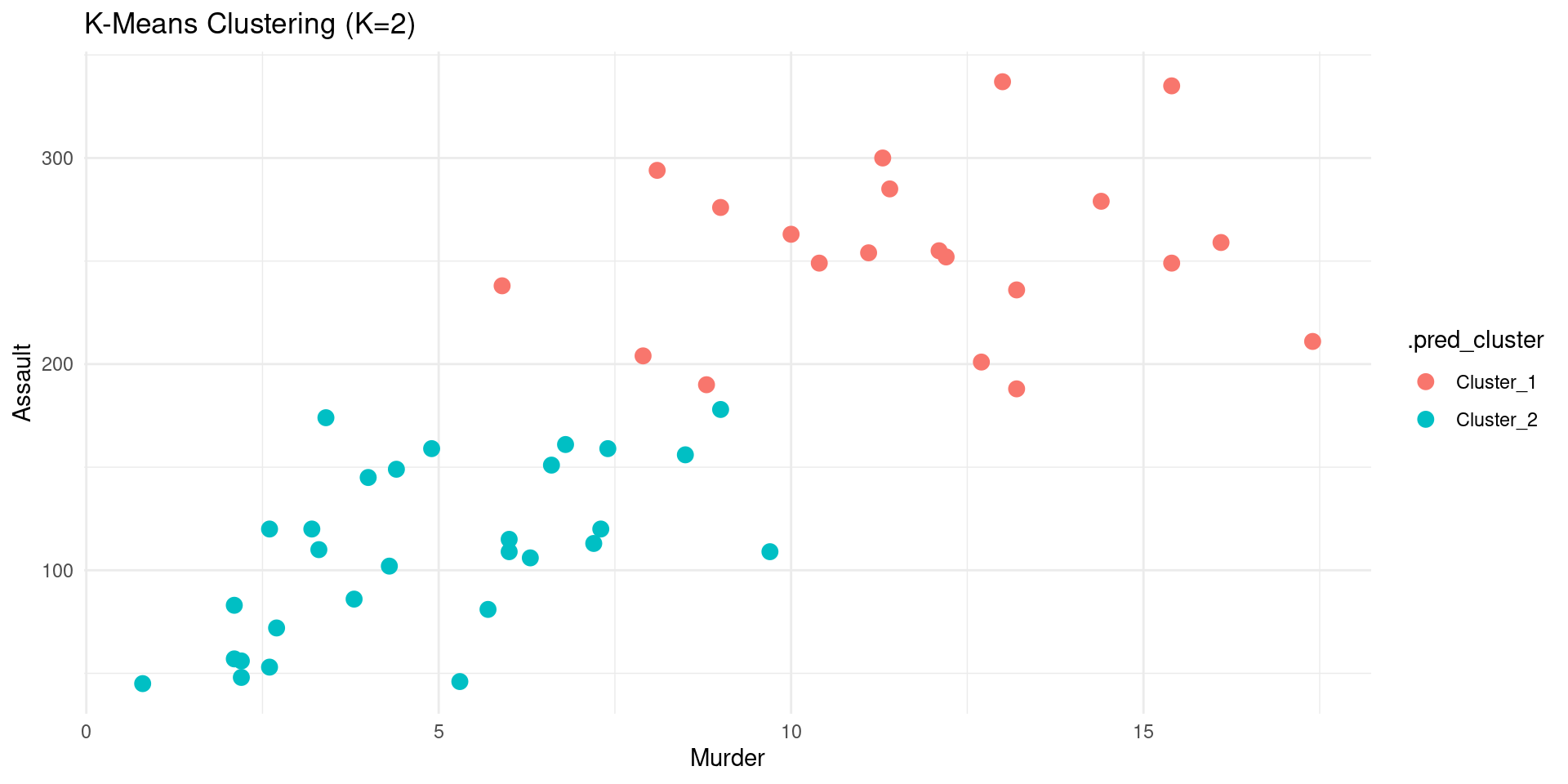      
2   4.84    110.     64.0  16.2    29   54762. 2

augment(kmeans_fit, USArrests) |>
  head()

# A tibble: 6 × 5
  Murder Assault UrbanPop  Rape .pred_cluster
   <dbl>   <int>    <int> <dbl> <fct>        
1   13.2     236       58  21.2 Cluster_1    
2   10       263       48  44.5 Cluster_1    
3    8.1     294       80  31   Cluster_1    
4    8.8     190       50  19.5 Cluster_1    
5    9       276       91  40.6 Cluster_1    
6    7.9     204       78  38.7 Cluster_1

Visualizing Clusters

With the cluster assignments, we can now visualize the clusters.

Code

kmeans_fit |>
  augment(USArrests) |>
  ggplot(aes(x = Murder, y = Assault, color = .pred_cluster)) +
  geom_point(size = 3) +
  labs(title = "K-Means Clustering (K=2)") +
  theme_minimal()

Visualizing Clusters PCA

We can also visualize the clusters in the PCA space.

Code

pca_rec <- recipe(~., data = USArrests) |>
  step_normalize(all_numeric_predictors()) |>
  step_pca(all_numeric_predictors(), num_comp = 2) |>
  prep()

US_Arrests_PCA <- bake(pca_rec, new_data = USArrests)

kmeans_fit |>
  augment(USArrests) |>
  bind_cols(US_Arrests_PCA) |>
  ggplot(aes(x = PC1, y = PC2, color = .pred_cluster)) +
  geom_point(size = 3) +
  labs(title = "K-Means Clustering (K=2)") +
  theme_minimal()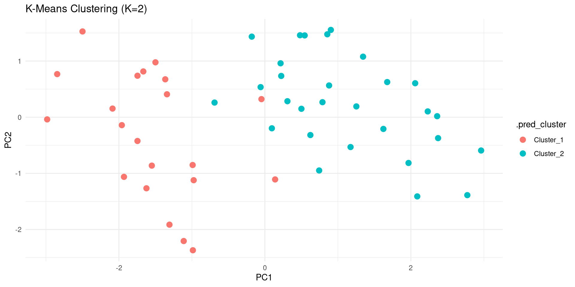

Tuning the number of clusters

How to choose the number of clusters K?
A common way is to try different values of K and see which one gives the best result.
We can use tune_cluster() to do this. Not this class.

Hierarchical Clustering

Another popular clustering method.
Creates a hierarchy of clusters, often visualized as a dendrogram.

How it Works (Agglomerative)

It’s a “bottom-up” approach:
1. Start: Each data point begins in its own cluster.
2. Merge: Find the two “closest” clusters and merge them into a single cluster.
3. Repeat: Repeat the “Merge” step until all data points are in a single cluster.
The history of merges forms the hierarchy.

Using `tidyclust`

Let’s do a hierarchical clustering with tidyclust.

hc_spec <- hier_clust() |>
  set_engine("stats")

hc_fit <- fit(hc_spec, ~., data = USArrests)

hc_fit

tidyclust cluster object


Call:
stats::hclust(d = stats::as.dist(dmat), method = linkage_method)

Cluster method   : complete 
Number of objects: 50

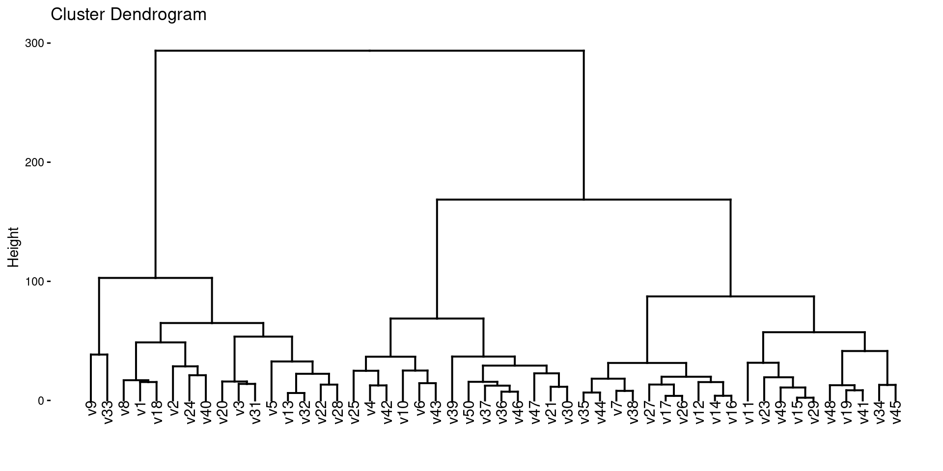
Dendrogram

The result of hierarchical clustering is often visualized as a dendrogram.
We can use the factoextra package to do this.

library(factoextra)

fviz_dend(hc_fit$fit)

Linkage

In hierarchical clustering, we need to specify a linkage method, which determines how the distance between clusters is calculated.
Common linkage methods are:
- complete: The distance between two clusters is the maximum distance between any two points in the two clusters.
- average: The distance between two clusters is the average distance between all pairs of points in the two clusters.
- single: The distance between two clusters is the minimum distance between any two points in the two clusters.

We can specify the linkage method in hier_clust().

hier_clust(linkage_method = "average")

Wrap-Up

Summary

Clustering: Finding groups in data.
K-Means: Partitions data into K clusters. Need to choose K.
Hierarchical Clustering: Creates a hierarchy of clusters.
tidyclust: A tidymodels-like interface for clustering.
tune_cluster() can be used to tune the number of clusters.

Do Next

(Optional)Read Chapter 12: Unsupervised Learning from ISLR.
There’s NO recitation Gem for this textbook but I recommend creating your own and adding the textbook chapter and these slides.
Move on to Lecture 34!

Unsupervised Learning

Unsupervised Learning

K-means Clustering

How it Works

tidyclust

The Data: USArrests

K-means with tidyclust

K-means with tidyclust

Understanding the result

Visualizing Clusters

Visualizing Clusters PCA

Tuning the number of clusters

Hierarchical Clustering

Hierarchical Clustering

How it Works (Agglomerative)

Using tidyclust

Dendrogram

Linkage

Wrap-Up

Summary

Do Next

`tidyclust`

The Data: `USArrests`

K-means with `tidyclust`

K-means with `tidyclust`

Using `tidyclust`